Parkinson’s and Huntington’s Disease x Voice Based Biomarkers: A-Two Part Project
This article will highlight how voice-based biomarker systems work, more about the emerging field and its need in the world, alongside two projects diagnosing Parkinson’s and Huntington’s disease. For more information on how these systems will help developing countries strive towards accessible healthcare, check out a previous article: Hey Alexa, What’s My Diagnosis. Githubs are linked throughout the article and videos can be found below:
A Broken Healthcare System
Our medical system around the world faces significant issues. Whether it be preventable medical errors, poor preventable mortality rates, lack of transparency in treatment, high costs of care, lack of insurance for low and middle class or lack of diagnosis supplies and list can go on and on and each of these aspects make up the broken healthcare system and all intertwine with each other.
Its a common misconception that these problems only occur in developing countries but really, each country faces their own problems. In particular, let’s take the United States as an example.
50 million people — 16% of the US population lacks health insurance coverage, meaning they have to pay extensive bills for healthcare, or they avoid going to the doctor at all.
In the US, the high cost of care is one of the country’s primary reasons for their broken system. The costs of new prescription drugs have risen and chronic illnesses in the US are at a higher number than many other countries yet contribute to the largest amounts of healthcare costs.
Patients with chronic illness spend 32% of total medicare spending, much of it going toward physician and hospital fees associated with repeated hospitalizations.
However, with telemedicine and remote monitoring on the rise, this combats part of the issue but not all of it. This is where voice based biomarkers come in. If we can reduce the amount of hospital visits and time spent at doctors offices or even diagnose these illnesses at an earlier rate, it can make a dent in the problem.
However, the problem doesn’t end there, because this is just one country.
Take for example, Malawi and their current healthcare conundrum. Over the past two years, the country has been facing major medical supply shortages due to their forex crisis, further inflating the prices of supplies. This in turn caused citizens to buy every medical supply they could, travel hundreds of miles to the central hospital and receive limited care.
No telemedicine could solve that problem.
However, every factor affecting the problem of access to healthcare relates back to money and resources some of which being preventable system inefficiencies.
For example, going back to the U.S, 30% of their healthcare spend is wasted but this goes for numerous countries (Figure 1). In fact, the top 15 healthcare countries waste between $1100 — $1700 USD per person, annually.
The average waste per person across the top 15 countries is 10–15x more than the average amount spent by the bottom 50 countries on healthcare, who currently spend $120/person. And, much of this extra hospital expenditure is due to mistakes in care or patients being infected while in hospitals.
In fact, some of these discrepancies are mind boggling. To really paint the picture, in seven low and middle income African countries, healthcare workers only make the correct diagnosis less than 45% of the time.
All of this goes to say that this universal problem is not an easy one to tackle and is multifaceted.
However, when systems become digital, the care becomes remote meaning there’s limited infections, minimal diagnosing errors, there’s no lack of human capacity and it’s much cheaper.
Digital Systems Will Override Top Doctors
Someday you will have better cardiac care in a village in India — which relies on an AI system — than at Stanford — which still relies on the cardiologists they just hired. The cardiologist will be an expert, but the AI will have 25 years of learning and improving every single day.
As many see these discrepancies in the system, a hypothesis is that improving the quality of care might mean removing humans from the loop.
Considering the status quo, here’s how a typical doctor’s visit looks like. Go to the doctors office → take loads of basic tests, majority are visual: tongue, throat, auditory, breathing → doctor assesses the situation → provides diagnosis → prescription received → send off.
This is in a safe and clean doctor’s office where the doctor inquires about your history and examines each system. However, this is a small percentage of doctors offices because in villages and developing countries, this isn’t the case.
But, instead of having invasive and high-tech tests, making this system completely virtual with high accuracy, accessibility and non-invasively, it can change the way healthcare is provided to the world.
Understanding the Voice
It might seem as an obvious reasoning behind the correlation of voice and certain organ systems, however, understanding the combination of speech analysis for health paired with machine learning is crucial to the basis of this project and emerging field.
To hear more about the machine learning correlation, refer back to this article to read more about acoustic and linguistic features and particular feature extraction from audio samples.
Now, every speech signal carries a bulk of information regarding the speaker in multiple ways. The linguistic content connects to the message the speaker is communicating and paralinguistic states and traits such as their current emotional states, age or gender.
The basis of vocal analysis is to break these signals down by these factors and features to then accurately recognize them, further diagnosing health conditions.
Speech production is a complex task and is specifically interconnected with physiological and cognitive systems, specifically respiratory and brain, as any slight changes in the speaker’s physical and mental states can affect their ability to control their vocal cords, causing fluctuations and altering their acoustic properties which can then be measured.
The anatomy of the human voice is unique in terms of its anatomical structure and its exact complexity of speech production which makes it a suitable marker for various health conditions. Specifically it requires the coordination of articulators (lip, tongue, jaw) and the respiratory muscles (diaphragm, larynx, etc). Plus, its the fastest human motor activity.
All of these aspects of the voice involve a large cognitive connection with message formation and memory and planning the articulatory movements to produce the intended sound, hence the causal relationship.
However, producing a sound is a multi step task. A simplified version of the process is when airflow from the lungs is created through exhalation is monitored by the oscillating movement of the vocal cords. During this step, the air exhaled from the lungs enters the glottis which contains the vocal folds. The sound source will then excite the vocal tract filter in turn, changing the positioning of the articulators, then changing the shape of the vocal tract. This change in shape then constructs the correct frequencies of the vocal tract filter.
Although the speed produced is different, the vocal tract properties and process remain the same.
Although the primary implementation of voice analysis has been built upon degenerative diseases, many health conditions and even human behavior can be analyzed such as fatigue, intoxication, cold/flu, respiratory diseases, etc. But, regardless of the application, there’s typically a concrete baseline system.
However, its important to note that there is no set in stone system which constitutes a “good” system performance as larger scale data is needed to establish a strong baseline.
A few basic features is the brute-forced feature extraction. This is feature extraction through the evaluation of combinations of input features and then finding the best subset as the test and currently have two main steps.
- Low Level Descriptions (LLDs) are extracted through a speech at frame rates of 25–40ms. These typically include pitch, energy and spectral descriptors for the spectrogram.
- The second step is applying functionals to each LLD to produce utterance summaries which form a single feature representation of an utterance.
All of that being said, there has been great research in the space with advancements emerging daily. However, to test out the correlation between neurodegenerative diseases and vocal cord fluctuations, I created two separate projects to highlight diagnosis of Parkinson’s and Huntington’s disease through vocal biomarkers. The remainder of this article will go through their features and code for the projects.
Parkinson’s <> Voice Analysis
Parkinson’s Disease (PD) is a degenerative neurological disorder caused by decreased dopamine levels in the brain. PD leads to the deterioration of movement, tremors, stiffness, changes in mood and changes in speech. In speech particularly, PD patients inherit dysarthria (a disorder where there’s difficulty articulating sounds), hypophonia (lowered volume) and monotone.
The status quo of diagnosing PD is a clinical will taker the neurological history of the patient and observe the patient’s motor skills in various situations. However, since there is no definitive laboratory test to diagnose PD, this part is difficult, particularly in the early stages when motor effects are not yet severe. Plus, monitoring progression of the disease over time requires repeat visits by the patient.
To avoid the frequent visits and to assist with early diagnosis voice recordings are a useful and non-invasive tool for diagnosis knowing that PD patients exhibit fluctuations in their vocal cords.
This way, rather than solely having qualitative observations to mark the diagnosis, there are quantitative approaches based on spectral and spectrogram analysis. This is a graph formed based on the frequencies extracted from a signal, allowing us to see abnormalities in specific vocal features such as fundamental frequency and HNR (harmonics to noise ratio).
The Github for this project alongside the dataset can be found here.
Before jumping into the code and focusing on the dataset, we can see that numerous features have been extracted to analyze and each column is vital.
- The name column highlights the patient’s name and recording number.
- MDVP:Fo(Hz) → Average vocal fundamental frequency, representing the vibratory rates of the vocal folds measured in hertz. The average Fo(Hz) for males ranges from 100 to 150 Hz, whereas for females it ranges from 180 to 250 Hz.
- MDVP:Fhi(Hz) — Maximum vocal fundamental frequency and highlights the oscillation occurring in the vocal folds during airflow produced through exhalation.
- MDVP:Flo(Hz) — Minimum vocal fundamental frequency.
- MDVP:Jitter(%) — highlighting the percentage of time during the audio sample where the patient’s frequency varied from cycle to cycle.
- MDVP:Jitter(Abs),MDVP:RAP,MDVP:PPQ,Jitter:DDP — Several measures of variation in fundamental frequencies.
- MDVP:Shimmer,MDVP:Shimmer(dB),Shimmer:APQ3,Shimmer:APQ5,MDVP:APQ,Shimmer:DDA — Several measures of variation in amplitude.
- NHR,HNR — Two measures of ratio of noise to tonal components in the voice.
- Status — Health status of the patient, 1 representing PD and 0 representing healthy.
The Code
We begin by first importing the necessary libraries.
#import libraries
import pandas as pd
import seaborn as sns
import matplotlib.pyplot as plt
%matplotlib inline
Next, we load the dataset and can see all of the extracted features from the output.
#loading the dataset
park = pd.read_csv('parkinsons.csv')
display(park.head())
print(park.shape)
Next, we further analyze the dataset to analyze patterns to extract major insights.
#finding patterns and insights in the data
display(park.describe().T)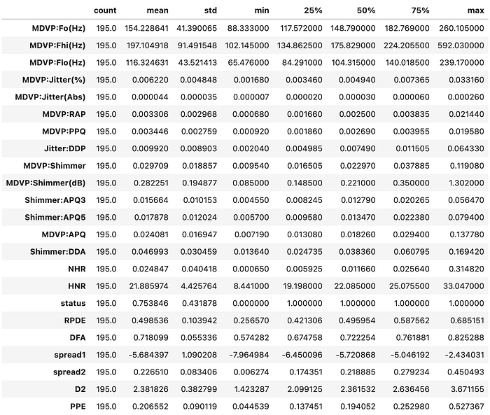
A few insights to extract are that some values are outliers as the mean is greater than the median and can mainly see a normal distribution across the dataset as the mean and median are fairly close to each other.
Then, we check the class imbalance to see if there’s specifically a greater representation of PD patients in the dataset by going through the status subsection and comparing the number of 1s to 0s.
#checking the class imbalance, specifically if there's a greater representation of people with Parkinsons in dataset
#.value_counts() goes through the data and checks which data is the most frequently occurring
print(park['status'].value_counts(normalize = 'True'))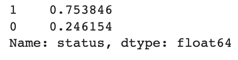
In this case, 75% of the dataset was with PD patients meaning there is a class imbalance and PD patients are overrepresented in the data.
Next, as a precautionary element, we check if there are any missing values from the feature extraction and from the result, we’ll see if there’s any imputing or removing needed.
#checking for missing values
print(park.isna().sum())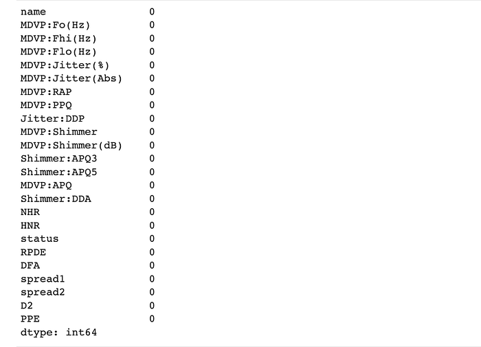
In this case, there were zero missing values.
Now, we move onto plotting the distribution of all the features with observations below.
#plot distributions of all the features based on pairwise distances and clusters
sns.pairplot(park, hue = 'status')
plt.show()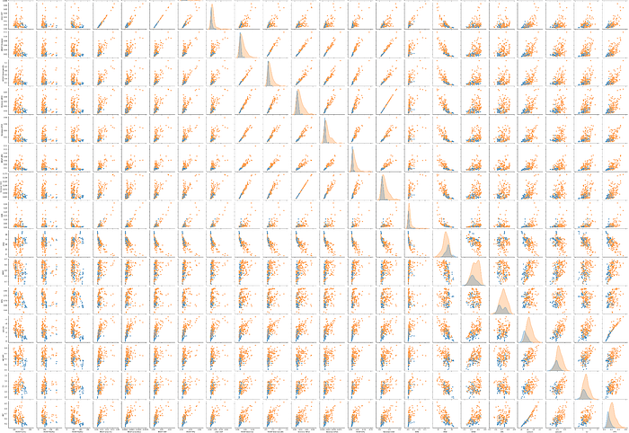
The main analyses collected are:
- Majority of the healthy patients have a higher value of Average Vocal Fundamental Frequency and Minimum Vocal Fundamental Frequency compared to the PD patients.
- NHR generally has higher values for PD patients and some outliers are also present in its distribution. On the contrary, HNR generally has higher values for healthy subjects with minimal outliers.
- DFA is approximately normally distributed for both the classes but for class 0 (Healthy) there are 2 distinct distributions.
Following the plots, we check for outliers in the data and if they are particularly high for any features. Considering that there are a total of 195 observations, certain features are considered to have greater outliers than others.
#checking for outliers, specifically how it varies from variable to variable
var = park.drop(['name', 'status'], axis = 1).columns
print('Number of outliers in different variables are\n')
for i in var:
    q1 = park[i].quantile(0.25)
    q3 = park[i].quantile(0.75)
    iqr = q3 - q1
    lw = q1 - 1.5 * iqr
    uw = q3 + 1.5 * iqr
    count = park[i][(park[i] < lw) | (park[i] > uw)].shape[0]
    print(f'{i}: {count}')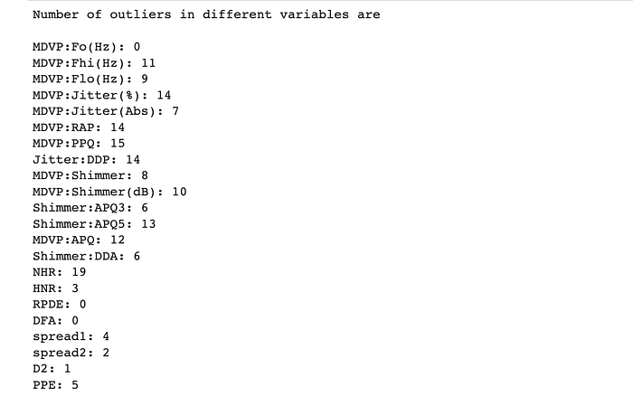
Then, we create a heatmap to analyze whether or not there are strong correlations between separate features.
#identifying correlations between the independent features from feature extraction
corr = park.drop(['name', 'status'], axis = 1).corr()
plt.figure(figsize = (20,20))
ax = sns.heatmap(corr, annot = True, cmap = 'icefire')
bottom, top = ax.get_ylim()
ax.set_ylim(bottom + 0.5, top + 0.5)
plt.show()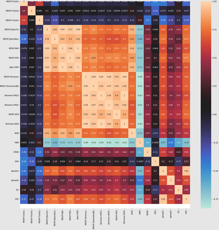
It is evident that the majority of the jitter and shimmer have strong correlations and all frequency related features relate back to the jitter and shimmer features.
Then we split the dataset into training the testing.
#splitting dataset into training and testing
X = park.drop(['name', 'status'], axis = 1)
y = park['status']
from sklearn.model_selection import train_test_split
X_train, X_test, y_train, y_test = train_test_split(X, y, test_size = 0.3, random_state = 3)
Through the dataset being split, we can now create a Random Forest Model which runs on the basis of forming multiple decision trees to create an accurate prediction.
#implementing random forest model to determine the optimal number of trees
from sklearn.model_selection import RandomizedSearchCV
from sklearn.ensemble import RandomForestClassifier
from scipy.stats import randint as sp_randint

rf = RandomForestClassifier(random_state = 3)
params = {'n_estimators' : sp_randint(50, 200)}
rsearch = RandomizedSearchCV(rf, param_distributions = params, n_iter = 100, scoring = 'roc_auc', n_jobs = -1,
                             cv = 10, random_state = 3, return_train_score = True)

rsearch.fit(X, y)
print(rsearch.best_params_)
However, in this case we are getting n_estimators to be 50 (the lowest limit that we had set) so now we will manipulate the numbers to arrive at an optimal value for the number of trees.
#for the n_estimators, 50 optimal trees was received so this was the lowest limit but now will run again to reduce
#the lower and upper limit to arrive at the optimal number of trees
rf = RandomForestClassifier(random_state = 3)
params = {'n_estimators' : sp_randint(25,75)}
rsearch = rsearch = RandomizedSearchCV(rf, param_distributions = params, n_iter = 50, scoring = 'roc_auc', n_jobs = -1,
                             cv = 10, random_state = 3, return_train_score = True)

rsearch.fit(X, y)
print(rsearch.best_params_)
#concluded that the optimal number of trees are 51 so are now fitting the model onto the optimal number of trees
from sklearn.metrics import accuracy_score, confusion_matrix, classification_report, roc_auc_score, roc_curve

rsearch.fit(X_train, y_train)

y_pred = rsearch.predict(X_test)
y_prob = rsearch.predict_proba(X_test)[:, 1]

print("Accuracy of Random Forest Model with optimal number of trees (51):", accuracy_score(y_test, y_pred))
print("\nConfusion Matrix:\n", confusion_matrix(y_test, y_pred))
print("\nClassification Report:\n", classification_report(y_test, y_pred))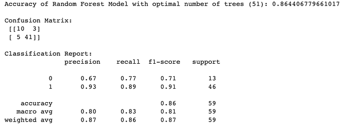
print("\nAUC Score:", roc_auc_score(y_test, y_prob))

fpr, tpr, _ = roc_curve(y_test, y_prob)
plt.plot(fpr, tpr, label = "AUC: " + str(roc_auc_score(y_test, y_prob)), color = 'b')
plt.plot(fpr, fpr, color = 'g')
plt.xlabel("FPR")
plt.ylabel("TPR")
plt.title("ROC Curve")
plt.legend(loc = 'best')
plt.show()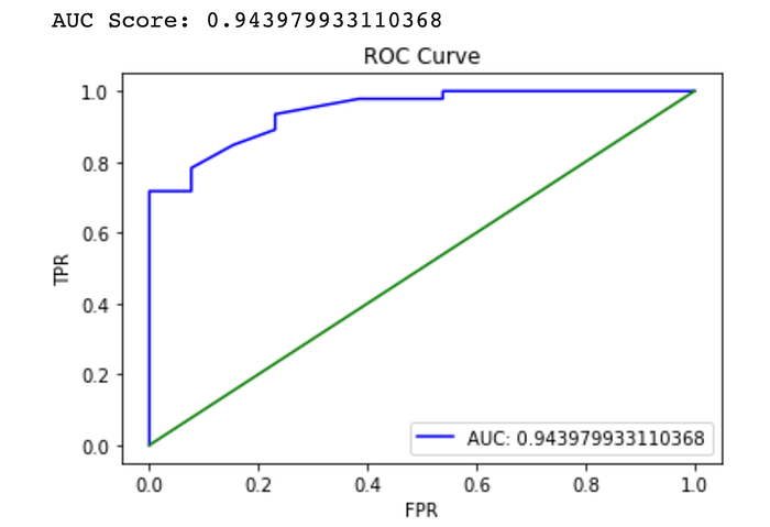
After fitting our model and receiving different matrices, we can see that the accuracy of the model is 94%.
Huntington’s <> Voice Analysis
Although similar to Parkinson’s, Huntingtons is another neurodegenerative disease, this disease is different as it’s genetic and causes the progressive breakdown and degeneration of nerve cells in the brain and one faulty gene causes part of your brain to damage gradually over time.
Like other degenerative diseases, Huntington’s (HD) causes motor and cognitive symptoms but has a clinical onset (earliest age when symptoms appear) of 45 years old and the symptoms gradually worsen.
In this case, there are two main sets of features.
- Phonatory features: relates to the larynx (voice box) and vocal folds.
- Modulation Power Spectrum feature (MPS): which is analyzing the variation of a simple signal by plotting the amount of energy of a particular temporal frequency (number of occurrences repeating per unit of time) and spectral frequency (the frequencies from each signal).
Both are useful, however, phonatory are used for finding optimal patients for clinical trials whereas MPS features assist with diagnosing. Regardless of the features analyzed, this system can help with three main problems. It will allow for early diagnosing, will speed up clinical trials and can expedite the process of understanding the disease.
Specifically with HD, we rely on the fact that patients suffering with HD have difficulty with speech and language production. HD patients have hyperkinetic dysarthria which is a subform of classic dysarthria where abnormal movements affect articulatory structures such as imprecise constants, phonation deviations and even a sudden forced breath.
The Github code and dataset for the project can be found here.
Patients in this dataset were recording the vowel “a” in a sustained manner for as long as possible, an acoustic analysis for three types of patients.
- C — Healthy patients
- preHD — carriers of HD (unaffected)
- HD — carriers and affected by HD
With HD, there are many dimensions and features to keep in mind. Here’s a quick breakdown.
Dimension: airflow insufficiency
- Feature 1: maximum phonation time which is the maximum amount of time someone can sustain a vowel for.
- Feature 2: first occurrence of a voice break is the first time a phonation stops.
Dimension: aperiodicity (periodic vibrations)
- Feature 1: number of voice breaks
- Feature 2: degree of pitch breaks which are the sudden shifts in high or low sections of speech.
- Feature 3: degree of vocal arrests
Dimension: irregular vibration of vocal folds
- Feature 1: F0 SD (standard deviation) highlights the frequency of the voice fundamental and its range in values for up to 2 SDs.
- Feature 2: recurrence period density entropy to analyze the repetitiveness of a signal.
Dimension: signal errors
- Feature 1: jitter (local) = average difference between two consecutive periods / the average period
- Feature 2: shimmer (local) = average difference between amplitudes of two consecutive periods / the average amplitude
Dimension: Increased noise
- Feature 1: harmonics to noise ratio (HNR)
- Feature 2: detrended fluctuation analysis which determines the statistical similarities in a signal
Dimension: signal errors
- Feature 1: jitter (local) = average difference between two consecutive periods / the average period
Dimension: vocal tremor (movement of muscles in the throat and larynx) and articulatory deficiency.
The Code
We begin the code by importing the necessary libraries.
#importing necessary libraries
from features import AudioSample
from pathlib import Path
import pandas as pd
from typing import List
! pip install librosa
import librosa
import numpy as np
We then load and store the audio samples, its sampling rate and the audio samples unique string id.
#Loading and storing the audio samples, its sampling rate (samples/second) and string id
samples_folder = Path('example_sound/')
audio_samples: List[AudioSample] = []
for wav_file in samples_folder.iterdir():
    if not wav_file.suffix == ".wav":
        continue
    else:
        audio_array, rate = librosa.core.load(str(wav_file), sr=44100)
        audio_samples.append(AudioSample(data=audio_array,
                                         rate=rate,
                                         name=wav_file.name))
Based on the features highlighted above, we then add all of the feature extractors for the audio files.
#adding all feature extrators for audio files
from typing import Dict

print('The DFA and RPDE are not computed by default.')
from features import *
compute_dfa_rpde = False
features_dict: Dict[str, SampleProcessor] = {
    "Maximum_phonation_time": MPT(),
    'Maximum_phonation_time_until_voice_break': MaximumPhonationUntilVoiceBreak(),
    'Aperiodicity_Features': AperiodicityFeatures(),
    'MFCCs_Mean_Of_Std': MFCCsMeanOfStd(),
    "hnr": PraatHNR(),
    "tremor": VocalTremorFeatures(),
    "signal_perturbation": PraatVoiceFeatures(),
    "mps": ModulationPowerSpectrumAnalysis(),
    "f0_stats" : FundamentalFrequency(method='shennong'),
}
if compute_dfa_rpde:
    features_dict["rpde"]= RPDE(dim=4, tau=35, epsilon=0.12, tmax=5000)
    features_dict["dfa"]= DFA(scale_boundaries=(1.259, 1.559), scale_density=0.03)
From there we can now build the extraction through a helper function that runs the extraction using the samples and the selected feature extractors. We can then use those onto our audio samples dataset.
#running a function which extracts the samples and selected features and will be stored
from collections import defaultdict
import tqdm

def extract(samples_list: List[AudioSample],
          features: Dict[str, SampleProcessor],
          fail_on_error: bool = True):
    #this function will run the extraction for each sample
    extracted_features = defaultdict(dict)
    for feature_name, processor in features.items():
        for audio_sample in tqdm.tqdm(samples_list):
            try:
                proc_output = processor(audio_sample)
            except Exception as e:
                if fail_on_error:
                    raise e
                else:
                    print(f"Got error on sample '{audio_sample.name}':' "
                          f"{type(e).__name__} :{str(e)}', skipping.")
            else:
                # maybe we should use tuples for the dict keys?
                extracted_features[audio_sample.name][feature_name] = proc_output

    return extracted_features

#run the extraction
extracted_features = extract(audio_samples, features_dict, fail_on_error=True)
We can format each of the features.
# Formatting the features
for file_name in extracted_features.keys():
    extracted_features[file_name]['Fraction of locally unvoiced frames'] = extracted_features[file_name]['Aperiodicity_Features']['Fraction of locally unvoiced frames']
    extracted_features[file_name]['Number of voice breaks'] = extracted_features[file_name]['Aperiodicity_Features']['Number of voice breaks']
    extracted_features[file_name]['Degree of voice breaks'] = extracted_features[file_name]['Aperiodicity_Features']['Degree of voice breaks']
    extracted_features[file_name]['Mean_Of_Std_mfcc'] = extracted_features[file_name]['MFCCs_Mean_Of_Std']['mfcc']
    extracted_features[file_name]['Mean_Of_Std_delta_mfcc'] = extracted_features[file_name]['MFCCs_Mean_Of_Std']['delta_mfcc']
    extracted_features[file_name]['frequency tremor intensity index (FTrI)'] = extracted_features[file_name]['tremor']['frequency tremor intensity index (FTrI)']
    extracted_features[file_name]['amplitude tremor intensity index (ATrI)'] = extracted_features[file_name]['tremor']['amplitude tremor intensity index (ATrI)']
    extracted_features[file_name]['jitter'] = extracted_features[file_name]['signal_perturbation']['jitter']['local']
    extracted_features[file_name]['shimmer'] = extracted_features[file_name]['signal_perturbation']['shimmer']['local']
    extracted_features[file_name]['F0_Std'] = np.std(extracted_features[file_name]['f0_stats'])

airflow_features_names = ['Maximum_phonation_time','Maximum_phonation_time_until_voice_break']
aperiodicity_features_names = ['Number of voice breaks','Degree of voice breaks','Fraction of locally unvoiced frames']
signal_perturbation_features_names = ['jitter','shimmer']
if compute_dfa_rpde:
    irregular_vibration_features_names = ['F0_Std','rpde']
    increased_noise_features_names = ['hnr','dfa']
else:
    irregular_vibration_features_names = ['F0_Std']
    increased_noise_features_names = ['hnr']
vocal_tremor_features_names = ['frequency tremor intensity index (FTrI)','amplitude tremor intensity index (ATrI)']
articulatory_features_names = ['Mean_Of_Std_mfcc','Mean_Of_Std_delta_mfcc']
all_features_names = airflow_features_names+aperiodicity_features_names+signal_perturbation_features_names
all_features_names += irregular_vibration_features_names+increased_noise_features_names
all_features_names += vocal_tremor_features_names+articulatory_features_names
classic_phonatory_features = {}
for file_name in extracted_features.keys():
classic_phonatory_features[file_name] = {curr_feat: extracted_features[file_name][curr_feat] for curr_feat in all_features_names}
classic_phonatory_features_df = pd.DataFrame.from_dict(classic_phonatory_features,orient='index')
len(classic_phonatory_features_df.columns)
There are many different signs when analyzing the audio samples however an HD gene carrier is considered premanifest (early stage) if they score less than five on both TMS (Total Motor Score) and their TFC (Total Functional Capacity) equals 13.
Now we can visualize the MPS features and look at the extracted features from the data.
#dataset description
classic_phonatory_features_df.describe()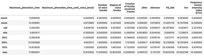
This next portion will create the plots from the extracted feature from each audio sample which can then be used to create the spectrogram for each patient.
#analyzing the MPS features and plotting for example audio samples
import matplotlib.pyplot as plt

def plot_mps(mps,wt,wf, DBNOISE=50):
    plt.figure()
    plt.clf()
    cmap = plt.get_cmap('jet')
    ex = (wt.min(), wt.max(), wf.min() * 1e3,
          wf.max() * 1e3)
    logMPS = 10.0 * np.log10(mps)
    maxMPS = logMPS.max()
    minMPS = maxMPS - DBNOISE
    logMPS[logMPS < minMPS] = minMPS
    plt.imshow(
        logMPS,
        interpolation='nearest',
        aspect='auto',
        origin='lower',
        cmap=cmap,
        extent=ex)
    plt.ylabel('Spectral Frequency (Cycles/KHz)')
    plt.xlabel('Temporal Frequency (Hz)')
    plt.colorbar()
    plt.ylim((0, wf.max() * 1e3))
    plt.title('Modulation Power Spectrum')
    plt.show()
Through this spectrogram we can analyze that the patient might be preHD as they are mainly clean with little voice breaks highlighting the warmer colours however to further the accuracy, a CNN can be used.
file_name = 'aaa_maureen.wav'
plot_mps(extracted_features[file_name]['mps']['mps'], extracted_features[file_name]['mps']['mps_wt'],extracted_features[file_name]['mps']['mps_wf'])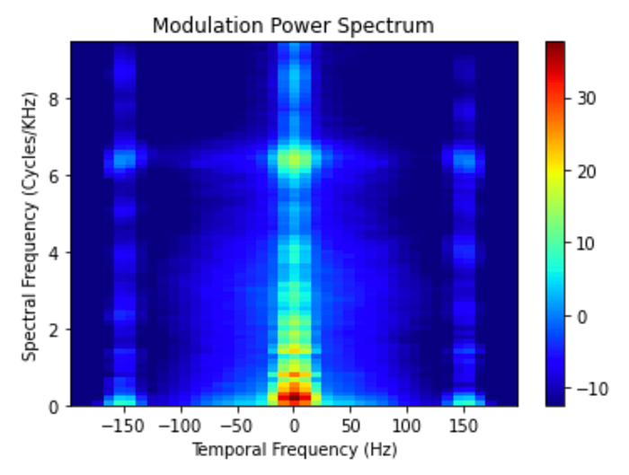
file_name = 'ah_mathieu.wav'
plot_mps(extracted_features[file_name]['mps']['mps'], extracted_features[file_name]['mps']['mps_wt'],extracted_features[file_name]['mps']['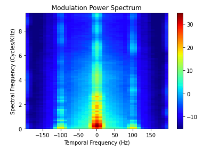
After analyzing degenerative diseases through vocal analysis, its clear that this system is possible but could use further development. Specifically, the lack of data or implementation in the space is hindering its growth.
However, with lots of R&D in the space of Parkinsons and degenerative diseases, the scope is high and maybe one day an AI will be training in a village in India for 25 years and be smarter than any doctor.